I do a lot of RSVP forms for work, using Google Forms. I’m finding that I’m sending out lots of invitations for “pick as many as you like” events – things like writing groups, workshop series, summer book clubs, all-day events where people can come and go.

Unfortunately, when you use checkboxes like this, Google Forms helpfully concatenates all the answers in a response. So it’s easy to tell what an individual has signed up for, but really hard to tell who’s signed up for the Thursday morning group.

If you don’t have too many options, or too many respondents, you can do some manipulation with Text to Columns and maybe a Transpose, but pretty soon I always find myself dragging data around on the sheet, a job that’s both tedious and error prone.

I suppose I could make each item on the form a “do you want this yes/no” radio button, but (a) that would be ugly and (b) I never remember this problem until I’m looking at data I can’t massage easily.

I was hoping to be able to handle this with a pivot table or a vlookup or some other function I don’t quite understand. These hopes all appear to be wrong, but searching for it is how I discovered the Filter function. That terrific linked page is where I learned that the Filter function can combine with the Search function, and critically, the Search function doesn’t require a complete match. It’ll find every instance of the searched-for text.

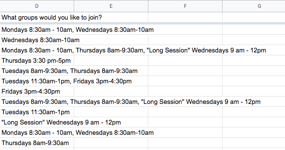
So, I opened a new tab in the results Google Sheet, and laid out all my options in the top row. (I’ve learned the hard way to always use different tabs for data and analysis.) To get a list of email addresses for each option, then I used this formula in each column.

=filter('Form Responses 1'!B:B,(search("SEARCH CRITERIA GOES HERE",'Form Responses 1'!D:D)))

Let’s take that apart. “Form Responses 1” seems to consistently be what Google Forms names the first tab of a responses Sheet. (If you’re not getting data through a Google form, well, change it to whatever the tab is called where your data lives.)

Column A is always a timestamp, and if you’re collecting email addresses they always go in B, so that’s why I’m filtering column B. If I wanted human names, in this form, I’d have used ‘Form Responses 1’!C:C

The Filter condition is the result of my Search against Form Responses 1, Column D, for matching responses… again, which column depends on how the form is organized. For the search criteria, I could have used a cell reference (A1, B1, C1…), since I did put all the options in Row 1 . That might have been better for cutting-and-pasting the formula or using it as a template for next year. I wanted it to be more human-readable, though, so my staff and I have a better chance of remembering how to do this in future.

Anyway, I hope writing this down helps me remember it, and maybe helps out other folks using Google Forms for RSVPs. Plus, I get to knock some dust off the blog.